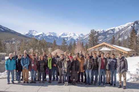
Thanks to everyone who made it to the Communication Complexity and Applications II workshop in Banff last month. See here for videos and here for open problems. Thanks to Sagar for compiling the open problems.

Ely asked me to remind everyone that the deadline for the 26th Annual Symposium on Combinatorial Pattern Matching is fast approaching. You have until 2nd February to match your combinatorial pattern.
Two of my students, Michael Crouch and Daniel Stubbs, are graduating this year. What does this mean?
Winner of the 2014 CRA Outstanding Undergraduate Research Awards!
This award “recognizes undergraduate students in North American colleges and universities who show outstanding research potential in an area of computing research.” Except, in Dan’s case, I’d skip the word “potential”.
Email me if you’d like to follow-up on any of the above points.
New Blog: Eric Blais, Sourav Chakraborty, and C. Seshadhri have started a new blog on property testing at http://ptreview.sublinear.info/. Also check out Moritz Hardt’s newish blog at http://mrtz.org/blog/.
This Blog: Things have been quieter at the polylogblog over the last few months but this will soon be rectified. This semester, I’m visiting the Simons Institute for the Theory of Computing in Berkeley. The program on Theoretical Foundations of Big Data Analysis has been great so far and the second workshop starts tomorrow: tune in live here for everything you’ve always wanted to know about “Succinct Data Representations and Applications”. However, with so much happening, I’ve been rather derelict in my blogging duties. Fortunately, numerous other bloggers have picked up the slack:
The exciting news sweeping the blogosphere (see here and here) is that SPARC 2013 is on its way. Specifically, Atri asked me to post the following:
Efficient and effective transmission, storage, and retrieval of information on a large-scale are among the core technical problems in the modern digital revolution. The massive volume of data necessitates the quest for mathematical and algorithmic methods for efficiently describing, summarizing, synthesizing, and, increasingly more critical, deciding when and how to discard data before storing or transmitting it. Such methods have been developed in two areas: coding theory, and sparse approximation (SA) (and its variants called compressive sensing (CS) and streaming algorithms).
Coding theory and computational complexity are both well established fields that enjoy fruitful interactions with one another. On the other hand, while significant progress on the SA/CS problem has been made, much of that progress is concentrated on the feasibility of the problems, including a number of algorithmic innovations that leverage coding theory techniques, but a systematic computational complexity treatment of these problems is sorely lacking. The workshop organizers aim to develop a general computational theory of SA and CS (as well as related areas such as group testing) and its relationship to coding theory. This goal can be achieved only by bringing together researchers from a variety of areas.
The Coding, Complexity and Sparsity workshop (SPARC 13) will be held in Ann Arbor, MI on Aug 5-7.
These will be hour-long lectures designed to give students an introduction to coding theory, complexity theory/pseudo-randomness, and compressive sensing/streaming algorithms. We will have a poster session during the workshop and everyone is welcome to bring a poster but graduate students and postdocs are especially encouraged to give a poster presentation.
This is the third incarnation of the workshop and the previous two workshops were also held in Ann Arbor in August of 2011 and 2012.
Confirmed speakers:
- Jin Yi Cai (University of Wisconsin, Madison)
- Shafi Goldwasser (MIT)
- Piotr Indyk (MIT)
- Swastik Kopparty (Rutgers University)
- Dick Lipton (Georgia Tech)
- Andrew McGregor (University of Massachusetts, Amherst)
- Raghu Meka (IAS)
- Jelani Nelson (Harvard)
- Eric Price (MIT)
- Christopher Ré (University of Wisconsin, Madison)
- Shubhangi Saraf (Rutgers University)
- Suresh Venkatasubramanian (University of Utah)
- David Woodruff (IBM)
- Mary Wootters (Michigan)
- Shuheng Zhou (Michigan)
We have some funding for graduate students and postdocs with preference given to those who will be presenting posters. For registration and other details, please look at the workshop webpage.

Ely Porat asked me remind everyone that the deadline for the 20th String Processing and Information Retrieval Symposium (SPIRE) is 2nd May, about a month from now. More details at websrv.cs.biu.ac.il/spire2013/.
Update: The deadline has been extended to 9th May.
A guest post from Krzysztof Onak:
A few recent workshops on sublinear algorithms compiled lists of open problems suggested by participants. During the last of them, in July in Dortmund, we realized that it would be great to have a single repository with all those problems. After followup discussions (with Alex Andoni, Piotr Indyk, and Andrew McGregor), we created a wiki page at http://sublinear.info/. Currently, it only contains open problems from the aforementioned workshops, but we invite submissions of inspiring problems from all areas of sublinear algorithms (sublinear time, sublinear space, etc.). Additionally, we want to compile a list of books, surveys, lecture notes, and slides that can be useful for learning about different areas of sublinear algorithms. We hope that this wiki will not serve only spambots, which have already been raiding it for a while, but it will also be a great source of inspiration for the whole community.
After a very successful hiring season last year, the department is now focusing on hiring in theory, NLP, robotics, and vision (that’s four separate searches rather than one extreme interdisciplinary position). So please apply! The official ad is here and note that, unlike previous years, we’re able to hire in theory at either the assistant or associate level. We’ll start reviewing applications December 3.

Continuing the report from the Dortmund Workshop on Algorithms for Data Streams, here are the happenings from Day 3. Previous posts: Day 1 and Day 2.

Michael Kapralov started the day with new results on computing matching large matchings in the semi-streaming model, one of my favorite pet problems. You are presented with a stream of unweighted edges on n nodes and want to approximate the size of the maximum matching given the constraint that you only have O(n polylog n) bits of memory. It’s trivial to get a 1/2 approximation by constructing a maximal matching greedily. Michael shows that it’s impossible to beat a 1-1/e factor even if the graph is bipartite and the edges are grouped by their right endpoint. In this model, he also shows a matching (no pun intended) 1-1/e approximation and an extension to a 
Next up, Mert Seglam talked about 


The next two talks focused on communication complexity, the evil nemesis of the honest data stream algorithm. First, Xiaoming Sun talked about space-bounded communication complexity. The standard method to prove a data stream memory lower bound is to consider two players corresponding to the first and second halves of the data stream. A data stream algorithm gives rise to a communication protocol where the players emulate the algorithm and transmit the memory state when necessary. In particular, multi-pass stream algorithms give rise to multi-round communication protocols. Hence a communication lower bound gives rise to a memory lower bound. However, in the standard communication setting we suppose that the two players may maintain unlimited state between rounds. The fact that stream algorithms can’t do this may lead to suboptimal data stream bounds. To address this, Xiaoming’s work outlines a communication model where the players may maintain only a limited amount of state between the sending of each message and establishes bounds on classical problems including equality and inner-product.
In the final talk of the day, Amit Chakrabarti extolled the virtues of Talagrand’s inequality and explained why every data stream researcher should know it. In particular, Amit reviewed the history on proving lower bounds for the Gap-Hamming communication problem (Alice and Bob each have a length n string and wish to determine whether the Hamming distance is less than n/2-√n or greater than n/2+√n) and ventured that the history wouldn’t have been so long if the community had had a deeper familiarity with Talagrand’s inequality. It was a really gracious talk in which Amit actually spent most of the time discussing Sasha Sherstov’s recent proof of the lower bound rather than his own work.
BONUS! Spot the theorist… After the talks, we headed off to Revierpark Wischlingen to contemplate some tree-traversal problems. If you think your observation skills are up to it, click on the picture below to play “spot the theorist.” It may take some time, so keep looking until you find him or her.

This week, I’m at the Workshop on Algorithms for Data Streams in Dortmund, Germany. It’s a continuation in spirit of the great Kanpur workshops from 2006 and 2009.

The first day went very well despite the widespread jet lag (if only jet lag from those traveling from the east could cancel out with those traveling from the west.) Sudipto Guha kicked things off with a talk on combinatorial optimization problems in the (multiple-pass) data stream model. There was a nice parallel between Sudipto’s talk and a later talk by David Woodruff and both were representative of a growing number of papers that have used ideas developed in the context of data streams to design more efficient algorithms in the usual RAM model. In the case of Sudipto’s talk, this was a faster algorithm to approximate 
Other talks included Christiane Lammersen presenting a new result for facility location in data streams; Melanie Schmidt talking about constant-size coresets for 


To be continued… Tomorrow, Suresh will post about day 2 across at the Geomblog.

Recent Comments